Subscribe to receive top agriculture news
Be informed daily with these free e-newsletters

Tough Decisions: Farmers are inundated with so much contradictory hedging advice that the concept morphs into a confusing mystery.
February 2, 2023

HEDGING QUESTIONS: Producers hear so many horror stories about hedging that they often turn away. But the reality is much more complex, and there are ways to improve your hedging decision making. Richard Hamilton Smith
by Cory Walters
Every year, the mantra “marketing is important” will be repeated from different points of view. Marketing services claim that preharvest marketing, or hedging, can help farmers increase their bottom line. Bank loan officers often imply that hedging can reduce price uncertainty, and agricultural economists join in by suggesting that hedging is a best management practice.
Producers, through either personal hedging experience or experience from other producers, smell the roses and feel the thorns. Horror stories about farmers losing money from hedging, or worse, losing their farm because “they played the futures market” circulate through rural communities.
Farmers are inundated with so much contradictory hedging advice that the concept morphs into a confusing mystery. Producers often respond by doing nothing, not because they think hedging is not important, but because they do not want to be wrong.
In this article, we connect what the industry says and what producers say to improve the disconnect and the decision-making environment associated with hedging. We accomplish this by inspecting the distribution of producer prices with and without hedging in the fall, as the distribution contains both yearly outcomes (producer concern) as well as the average outcome (another point of view).
Computer models are used to lift the mystery surrounding the role of hedging. Computer models help understand complex processes, allowing for a better decision environment, leading to improved financial standing and stability. Our model reproduces the risk profile that individual farmers experience. We accomplish this through a holistic view where we inspect hedging performance through the lens of a larger context — the evolution of prices before prices are observed. We are thinking of the 2023 crop year.
Click through the gallery to see a summary of our results and graphs to explain the data, along with a description of our approach.
We first lay out the framework in which decisions will be made. First, fall prices will be revealed when we get to the fall, and we cannot predict fall price beforehand. Second, the hedging decision happens before the fall price is known, so we must make the decision looking into an unknown future. Third, the path in which prices evolve from the spring to the fall will be unique.
There are thousands of possible price paths, yet we see only one each year. It is here, the path prices take that matters so much. We only observe one price path per year, but there exist thousands of possibilities. Fourth, probability of 2023 corn futures price path being like 2022 is close to zero.
What do we do? We model price evolution of thousands of potential paths by allowing prices to evolve through random shocks. Shocks could reflect wars, production issues, etc. We then include hedging into this model and observe the changes in price outcomes. Here, price outcomes are defined as the average farm price since the farm sells some crop through the hedge and the rest at harvest.
The time period we are considering here is from March 1 to Nov. 1, the preharvest time frame. For simplicity, we are focusing on daily moves. Each day, the farmer can sell at the closing price or wait until the next day for new closing price. For example, on March 1, the market absorbs the available supply and demand information and establishes a consensus price that represents an equilibrium between potential buyers and sellers. On March 1, the farmer has the choice to sell some, or all, of their anticipated production at the price the market offers or wait until the next day. As new information arrives, the market adjusts. The farmer can accept the new market consensus by pricing part of their crop or wait for a possibly better offer the next day.
This leads to a daily recurrent process continuing until the history of sales along a particular time-dependent path is tallied at a preset ending point, Nov. 1 in this analysis. Sales occur along a possible path. With this, we assume that Ln prices meander through time following a Generalized Browning Motion Stochastic Model:
(1) ∆ [Ln(P)] = (μ – σ^2/2) ∆t +σ ε(∆t)^(1/2)
In this equation, ε represents the standard normal distribution, μ represents the drift, σ represents the implied volatility. This process represents a simple explanation of the marketing mystery. Each day, the price changes by the deterministic first term and a random part that represents new information arriving in the marketplace.
Monte Carlo estimates the results implied by Equation 1 by sampling this equation with many different paths. Each path experiences a different random exposure to information each day. Historical seasonality (i.e., piecewise drift) is added to the model framework and the resulting differential equation is solved numerically. Today's computers and the availability of modern software applications, such as Analytica, make it possible to conduct this intensive numerical calculation. This improved technology lets the producer do the thinking while the computer does the work.
When tested using historical yearly data, Zimmerman et. al. 2021 found that a marketing plan based on selling a certain amount of production at fixed times throughout the year outperformed sell nothing until harvest plan as well as multiple other marketing plans.
Ed Usset clearly how different marketing plans have performed in his introduction to marketing, “Grain Marketing is Simple (It’s Just Not Easy).” We can incorporate this marketing plan into our stochastic model. Using this “timed” method, known as Terry Timer, we make 10 equally sized sales 10 days apart on each path.
To simplify the complexities of farm management decision making, agricultural economists often present hedging as a separate enterprise. Once it is separated it is assumed that hedging is recommended if it produces a profit. In this reductionist view, hedging value is measured as the difference of selling expected production using a marketing plan or not, given by
Hedge Value(n)= Market Plan(n)- Fall Price(n)
for each possible path n. Often, for simplicity, only the average is reported. (See Figures 3, 4 and 5 in gallery for more explanation.)
Hedging influences your farm average price. We encourage you to focus on this viewpoint. Not that we are encouraging you to engage in hedging, as this is a personal decision, rather, that when you are deciding whether to hedge, base the decision on creating a farm average price.
While our focus was on hedging, production risk also exists. While a hedge sets a price, which reduces uncertainty, it increases production risk. If production falls short of the amount hedged and the fall price turns out higher than the average hedge price, these shortfall bushels must be bought back at the higher price. This is an added risk introduced by hedging, an unintended consequence. Limiting hedging to a percent of expected production and purchasing a revenue-based crop insurance policy at a reasonable coverage level provides financial protection from buying back contracts.
Walters is an associate professor in the department of agricultural economics at the University of Nebraska-Lincoln.
You May Also Like
Enter a zip code to see the weather conditions for a different location.